September 2016

(Note: all the previous publications in the basic statistics category are listed on the right-hand side.  Select "Return to Categories" to go to the page with all publications sorted by category.  Select this link for information on the SPC for Excel software.)

As part of your PPAP process, you have to provide a process capability analysis to your customer for the trial production run you just completed.  The histogram of the data you collected does not look normally distributed.   A normal probability plot confirms your fears – you are dealing with non-normal data.  You run a Box-Cox transformation to see if the data can be transformed into a normal distribution.  The transformation does not work.  Now what do you do? 

A process capability analysis requires a normal distribution to be able to calculate a Cpk value.  You will not be able to use Cpk.  You will have to do a non-normal process capability analysis.  But to perform that analysis, you have to determine what distribution best fits your data.

This publication explains how distribution fitting is done using the exponential distribution as an example.  Next month’s publication will expand this to compare multiple distributions to see which distribution fits your data the best.

In this issue:

• What is Distribution Fitting?
• Not Everything Fits a Normal Distribution
• Identifying the Best Distribution
• Distribution Parameters
• Parameter Estimation
• Example
• Is the Fit Any Good?
• Summary
• Quick Links

Please feel free to leave a comment at the end of this publication.  You may also download a pdf copy of this publication at this link.

What is Distribution Fitting?

Distribution fitting is the process used to select a statistical distribution that best fits the data.  Examples of statistical distributions include the normal, gamma, Weibull and smallest extreme value distributions.  

In the example above, you are trying to determine the process capability of your non-normal process.  This means that you need to be able to define which distribution fits the data best so you can determine the probability of your process producing material beyond the specifications.  It is important to have the distribution that accurately reflects your data.  If you select the wrong distribution, your calculations will be wrong.

Just a brief note on the data itself.  The data should be consistent and predictable, i.e., it should have been generated from a process that is in statistical control.  If the process is not in statistical control, the distribution fitting will not be accurate.

Not Everything Fits a Normal Distribution

Life would be great if we could just assume that our data were normally distributed.  It is the most frequently used distribution.  Why?  Because many things are normally distributed.  But not everything.  The normal distribution is defined by the average and standard deviation.  It is symmetrical about the average.  

Distributions that are skewed to the left or to the right cannot be modeled as normal distributions.  Other distributions are bounded and cannot be modeled as normal distributions.  And there are symmetrical distributions that may fit your data better than a normal distribution does.

Picking the wrong distribution gives you inaccurate results.  Our previous publication on non-normal process capability provides an example of how your process capability calculations for Cpk are not correct if don’t have a normal distribution.

Identifying the Best Distribution

Multiple distributions are usually tested against the data to determine which one fits the data the best.  You can’t just look at the shape of the distribution and assume it is a good fit to your data.

How do you determine the best distribution?  Statistical techniques are used to estimate the parameters of the various distributions.  Once this estimation is complete, you use goodness of fit techniques to help determine which distribution fits your data best.  There are also visual techniques that help you decide which distribution is best.  These includes examining a histogram with the distribution overlaid and comparing the empirical model to the theoretical model.   These methods are examined in more detail below.

Distribution Parameters

The distribution's parameters define the distribution.  There are four parameters primarily used in distribution fitting.  These four parameters are:

• Location
• Scale
• Shape
• Threshold

Not all parameters exist for each distribution.  For example, the normal distribution has only two parameters: location (the average) and scale (the standard deviation).  These two parameters completely define the normal distribution.  Distribution fitting involves estimating the parameters that define the various distributions.  The four parameters are defined in more detail below.

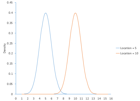
The location parameter of a distribution indicates where the distribution lies along the x-axis (the horizontal axis).  Figure 1 shows two normal distributions.  The location values are different.  The blue distribution has a location of 5.  The orange distribution has a location of 10.  Both have the same standard deviation (or scale in parameter terms).

Figure 1: Normal Distribution with Different Locations

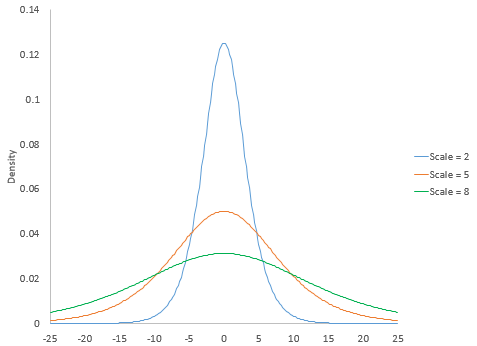
The scale parameter of a distribution determines how much spread there is in the distribution.  The larger the scale parameter, the more spread there is in the distribution.  The smaller the scale parameter, the less spread there is in the distribution.  Figure 2 shows the logistic distribution with three different scale parameters: 2, 5, and 8.  The location for all three curves is 0.

Figure 2: Logistic Distribution with Different Scale Parameters

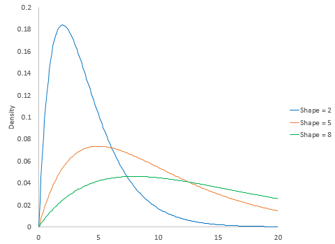
The shape parameter of a distribution allows the distribution to take different shapes.  The two distributions above, the normal and the logistic distributions, do not have a shape parameter.  The shape is defined by the location and scale for these two distributions.  Other distributions have shape parameters.  The larger the shape parameter, the more the distribution tends to be skewed to the left.  The smaller the shape parameter, the more the distribution tends to be skewed to the right.  Figure 3 shows how changing the shape parameter impacts the gamma distribution.  The scale parameter for the gamma distribution in Figure 3 is 2.  The gamma distribution does not have a location parameter.

Figure 3: Gamma Distribution with Different Shape Parameters

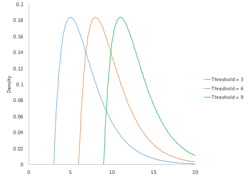
The threshold parameter of a distribution defines the minimum value of the distribution along the x-axis.   The distribution cannot have any values below this threshold.  Figure 4 is the gamma distribution with three different threshold values: 3, 6 and 9.  The scale and shape parameter are both 2.

Figure 4: Gamma Distribution with Different Threshold Values

Parameter Estimation

A number of statistical techniques can be used to estimate the parameters for a distribution.  SPC for Excel uses the maximum likelihood estimation (MLE) technique.   We will use the exponential distribution as an example.  

The exponential distribution is a commonly used distribution in reliability engineering and is used to model the time between failures when the units have a constant failure rate.  This distribution has one parameter and there is an analytical solution for finding that parameter.  Suppose we have a sample of size n from a single distribution.  We want to know if the sample came from an exponential distribution.

You begin with the probability density function (pdf) for the distribution.  The exponential pdf is given by:

where b is the scale parameter; b must be greater than 0.  Our objective is to find the value of b based on our sample data.  Each x_i has the same pdf since the samples come from the same distribution.

The likelihood function of a random sample, L, is defined as the product of each individual pdf:

Substituting in the exponential pdf gives:

We want to find the value of b that maximizes this likelihood function.  Here is the trick with MLE.  It is easier to minimize the negative log likelihood.   Taking the negative log of both sides of the above equation converts the product of the pdfs to the sum of the pdfs:

Substituting in the exponential pdf gives:

The above expression can be simplified to the following:

We want to find the value of b that minimizes this function.  To find this, you take the partial derivative of -ln L with respect to b and set that equation to 0.

Solving for b gives the following:

This is simply the equation for the average.  For the exponential distribution, the scale parameter that is equal to the average minimizes the log likelihood function.  

This is the MLE approach.  The calculations become more difficult for most other distributions.  The log likelihood function has to be differentiated with respect to each parameter being estimated with each of the resulting equations set to zero.  Then the equations must be solved simultaneously to find the distribution's parameters.  Numerical methods must be used for most distributions. 

Example

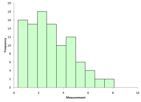
Suppose we have sample of 100 data points.  You can download the data used at this link.  A histogram (Figure 5) of the 100 data points show that the data are not normally distributed.  

Figure 5: Histogram of Sample Data

Normally, multiple distributions are tested to determine which fits the data best.  For this publication, we will just use the exponential distribution.  We have already shown that the minimum of the log likelihood function for the exponential distribution occurs when the scale parameter b equals the average.  

The average of the data set is 2.975.  So, the exponential pdf becomes:

We have defined the exponential distribution based on our data.  But how good does it fit the data?

Is the Fit Any Good?

We know from above that, when the scale parameter equals the average, the log likelihood function is minimized and this is the best fit for the exponential distribution.  But is that fit any good?  

There are a number of ways of judging goodness of fit.  A very common way is to calculate the Anderson-Darling statistic and determine the p-value associated with that statistic.  The test assumes that the data fits the specified distribution.  A low p-value means that assumption is wrong and the data does not fit the distribution.  A high p-value means that the assumption is correct and the data does fit the distribution.

An earlier publication covered how to calculate the Anderson-Darling statistic for the normal distribution.  The process is the same for other distributions except that you use the cumulative distribution function (CDF) for that distribution in the calculations.  The data were analyzed using the SPC for Excel software and the following results were obtained for the exponential distribution:

• Anderson-Darling statistic = 6.374
• p-value < 0.001

Since the p-value is so small, you conclude that the exponential distribution does not fit the data.

There are also visual methods you can use to determine if the fit is any good.  One is to overlay the pdf for the distribution on the histogram of the data.  This is shown in Figure 6.

Figure 6: Histogram with Exponential pdf

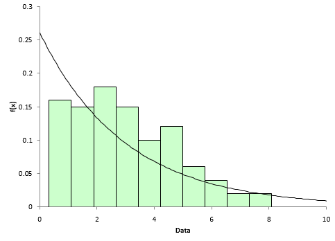
The exponential distribution does not appear to fit the data very well based on Figure 6.

Another visual way to see if the data fits the distribution is to construct a P-P (probability-probability) plot.  The P-P plots the empirical CDF values (based on the data) against the theoretical CDF values (based on the specified distribution).  The CDF for the exponential distribution is given by:

If the P-P plot is close to a straight line, then the specified distribution fits the data.  Figure 7 shows the P-P plot for the data against the exponential distribution.

Figure 7: P-P Plot for Exponential Distribution

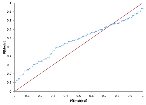
The data in Figure 7 does not fall along a straight line – more evidence that the exponential distribution does not fit the data.

Summary

This publication has introduced distribution fitting.  Distributions are defined by parameters.  The various parameters (location, scale, shape and threshold) were introduced.  The maximum likelihood estimation method is used to estimate the distribution's parameters from a set of data. The exponential distribution was used an example.  Methods of checking how “good” the distribution matches the data were also introduced.  These goodness of fit methods include the Anderson-Darling statistic, comparing the histogram to the probability density function, and constructing a P-P plot to compare the theoretical cumulative density function to the empirical cumulative density function.  Our next publication will examine how to compare multiple distributions when trying to find a distribution that best fits the data.